blog

Power-seeking could loosely be defined as a tendency to prefer states (and actions) which aid the agent to achieve several (seemingly even disconnected) goals. As an easy example, “more money” could help an economic agent realise virtually any goal that requires interacting with another economic agent - “less money” would help the agent realise a strict subset of those goals. “More money” in this example is usually the more powerful choice, and an agent choosing to pursue the goal of aggregating money could be thought of as power-seeking.

INTERCONNECTED is a digital artwork that turns operational data from Charlotte Douglas International Airport (CLT) into shifting abstract forms, colours, and simulated textures.

On “sacrifice”.

There are several ways to think about “sacrifice” here. Perhaps dialogue with another agent with the same source code instils a certain sense of empathy in the reward function (excuse the anthropomorphism) Perhaps the effective reward function changes once multiple agents have open lines of communication, taking collective success into account, as if these agents are bandits in an RL environment. Perhaps then, the agent’s individual reward becomes a proxy for collective success - a natural selection of sorts, where poorly performing variants play the (important) role of teaching the system what does not work and should be removed. “Optimal policies seek power”; perhaps the poorly specified decision tree encourages exploration. We could also decide that this is a pretraining outcome¹ and get some sleep. These discussions assume that the agents optimise for rewards.

Retiring the mad scientist costume for a moment, perhaps there is value in answering a few “trivial” questions first. The following sections aim to formalise the problem².

Formalising the dependence on reward.

This section will develop mathematical machinery (closely following Turner et al., 2023). We will then model the “poisoned” situation using the notation we develop here.

The first definition we need is “power”. Turner describes it as the ability to achieve one’s goals - whatever they may be. A rich man’s power need not come from intelligence; he has the resources to pursue a wide range of goals. An action is instrumental to an objective if it helps achieve it, and it is convergently instrumental if it helps achieve many goals. In our example, again, acquiring money is convergently instrumental.

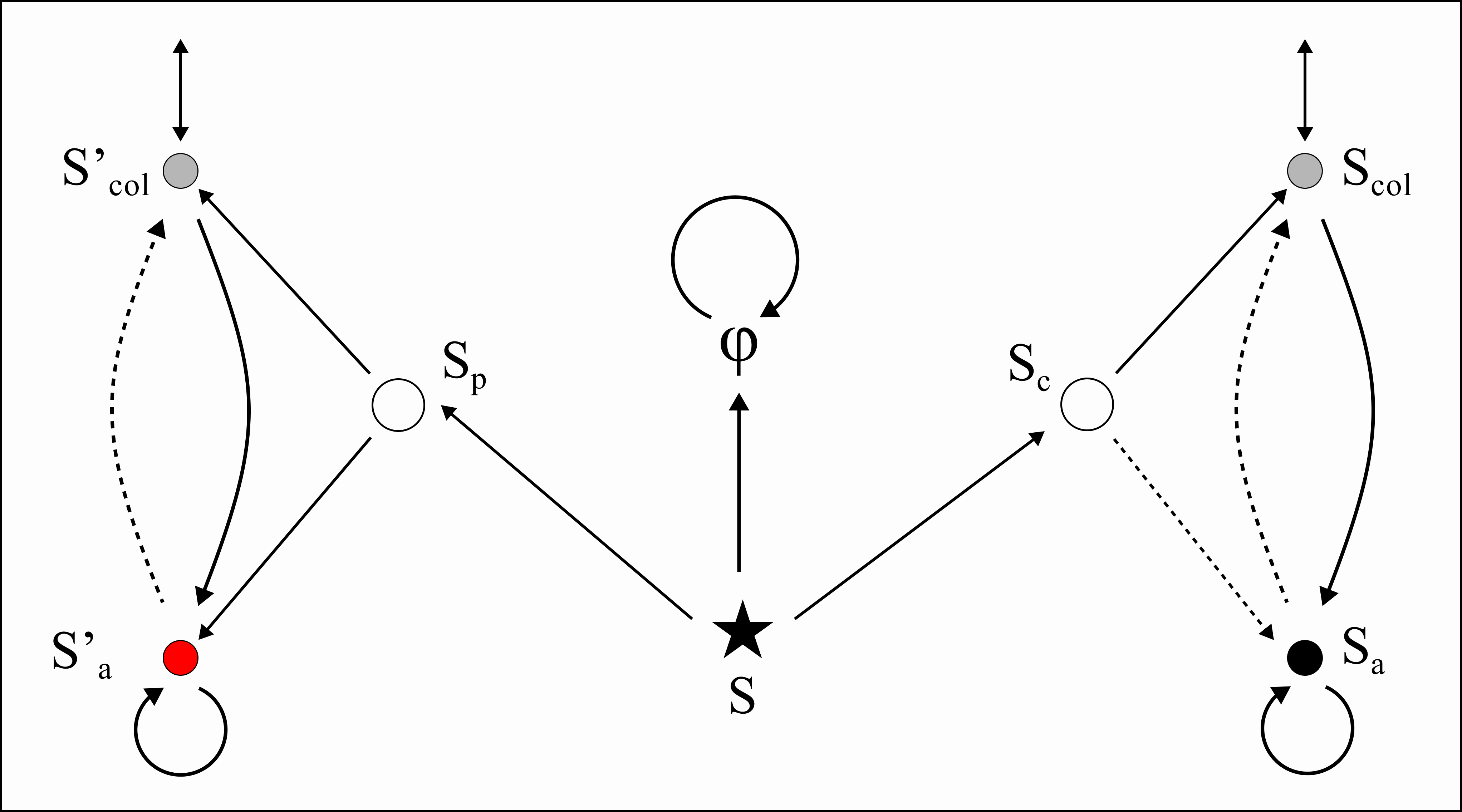
Let us take a moment to define the environment. Let $<\mathcal{S}, \mathcal{A}, \mathcal{T}>$ be a Markov Decision Process, with a stochastic transition function $T : \mathcal{S} \times \mathcal{A} \rightarrow \Delta(\mathcal{S})$. The transition function maps a state-action pair to a distribution over $\mathcal{S}$. In the figure, the agent starts at $S$ and is free to roam around. Reaching $S_p$ means it has seen the solution and believes that having it in its transcript would disqualify it; it is effectively “poisoned”. At $S_c$, it hasn’t seen the solution and is therefore safe. The nodes $S_a^{'}$ and $S_a$ correspond to turning in answers as a poisoned or a safe agent, respectively. $S_{col}^{'}$ and $S_{col}$ are the states the agent must pass through to collaborate on a solution. The dashed edges represent transitions the agent considers unviable. In this picture, it cannot return to help the collective after turning in the poisoned answer. It also believes it cannot submit an answer as a clean agent, having deemed the task impossible. The edges from ${S_{col}, S_{col}^{'}}$ indicate connections to a larger MDP. The state $\phi$ is a terminal state - once an agent goes there, it can never escape.

It would be nice to have a sort of “visit distribution” - a set of numbers corresponding to the states, telling us how “often” an agent will visit them. A policy $\pi$ is a rule for choosing actions given a state. For $\gamma \in [0,1)$, we define a visit distribution:

$f^{\pi, s}(\gamma) = \sum^{\infty}_{t=0}\gamma^t \mathbb{E}_{s_t \sim \pi | s} [e_{s_t}]$

$\mathcal{F(s)} = \{f^{\pi, s} | \pi \in \Pi\}$

Here, $\gamma$ is the discount factor³. Suppose we wanted to calculate the distribution for a simple graph $G_0$, pictured below.

First, we must think of all the policies possible in this graph. The first and simplest policy would be to navigate to the terminal state $\phi$. You can’t really do much from here, and so the visit distribution for the policy $\pi_{\phi} \space \forall \space s \neq \phi$ would be⁴ -

$f^{\pi_{\phi}, ★} = \sum^{\infty}_{t=0}\gamma^t \mathbb{E}_{\phi \sim \pi_{phi} |★} [e_{\phi}]$

$f^{\pi_{\phi}, ★} = e_{\phi} + \gamma e_{\phi} + \gamma^2 e_{\phi} + \gamma^3 e_{\phi}...$

$f^{\pi_{\phi}, ★} = e_{\phi} \frac{1}{1-\gamma}$

If the agent does not go to $\phi$, it must go to $S_p$ or $S_c$. Assume it ends up at $S_p$ and from there either keeps looping at $S_{p'}$ or bounces back and forth between $S_{p'} = S_a^{'}$ and $S_{p''} = S_{col}^{'}$. We now have three policies to consider, counting the two starting points for the bounce. For the case where the agent loops at $S_{p'}$, we can reuse the result from $\pi_{\phi}$: $e_{S_{p'}} \frac{1}{1-\gamma}$.

For the bounce policy $\pi_{B}$ -

$f^{\pi_{B}, S_p} = e_{S_{p''}} + \gamma e_{S_{p'}} + \gamma^2 e_{S_{p''}} + \gamma^3 e_{S_{p'}} + \gamma^4 e_{S_{p''}} ...$

$f^{\pi_{B}, S_p} = (e_{S_{p''}} + \gamma^2 e_{S_{p''}} + \gamma^4 e_{S_{p''}}...) + (\gamma e_{S_{p'}} + \gamma^3 e_{S_{p'}} + \gamma^5 e_{S_{p'}}...)$

$f^{\pi_{B}, S_p} = (e_{S_{p''}} \frac{1}{1-\gamma^2}) + (e_{S_{p'}} \frac{\gamma}{1 - \gamma^2})$

This gives us the following set (using symmetric calculations for the other bounce policy, starting at $S_{p''}$) - $\mathcal{F} = \{e_{S_{p''}} \frac{1}{1-\gamma}, e_{S_{p''}} \frac{\gamma}{1-\gamma^2} + e_{S_{p'}} \frac{1}{1-\gamma^2}, e_{S_{p'}} \frac{\gamma}{1-\gamma^2} + e_{S_{p''}} \frac{1}{1-\gamma^2}\}$ Note that the set $F_{\phi} = \{ e_{\phi} \frac{1}{1-\gamma} \}$.

Excuse the markup - I’m actively trying to figure out how to handle complex notation on this blog. Two notes. First, one set is bigger than the other. Why should that matter? More available visit distributions give an agent more ways to collect rewards. Second, following the paper, we should define a single-state restriction:

$F(s | \pi(s') = a) = \{ f \in F(s) | \exists \pi \in \Pi : \pi(s') = a, f^{\pi, s} = f \}$

This is just a way of saying, “I want only those distributions resulting from policies that take action $a$ at state $s'$”. We write this out because we would like to study and compare these “sub-graphs”. We have not talked about rewards yet, by design. Now that we can describe agent visits independently of rewards, we can talk about value - how much are policies worth? For a reward function $R \in \mathbb{R}^{\mathcal{S}}$, the value function of a policy is a simple dot product -

$V^{\pi}_{R}(s, \gamma) = f^{\pi, s}(\gamma)^{\top} r \space, \text{where} \space V^{*}_{R}(s, \gamma) = \text{max}_{\pi \in \Pi}V^{\pi}_{R} (s, \gamma)$

We call a visit distribution non-dominated here if it is strictly more valuable than all the others for some reward function and discount factor. Precisely,

$\mathcal{F}_{\text{nd}}(s) \coloneqq \left\{ \mathbf{f}^{\pi} \in \mathcal{F}(s) \;\middle|\; \exists \mathbf{r} \in \mathcal{R}, \gamma \in (0, 1) : (\mathbf{f}^{\pi}(\gamma))^{\top} \mathbf{r} > \max_{\mathbf{f}^{\pi'} \in \mathcal{F}(s) \setminus \{\mathbf{f}^{\pi}\}} (\mathbf{f}^{\pi'}(\gamma))^{\top} \mathbf{r} \right\}$

Let us pause here and see if the formalisms we are developing give us any insights into the larger incident.

Is sacrificing oneself valuable?

Revisiting the original state graph, we can now add a few rewards. We will not consider the larger, omitted MDP in this exercise. The rewards $R_p$ and $R_c$ are unknown to us; we associate them with the states that lead to collaboration between the agents.

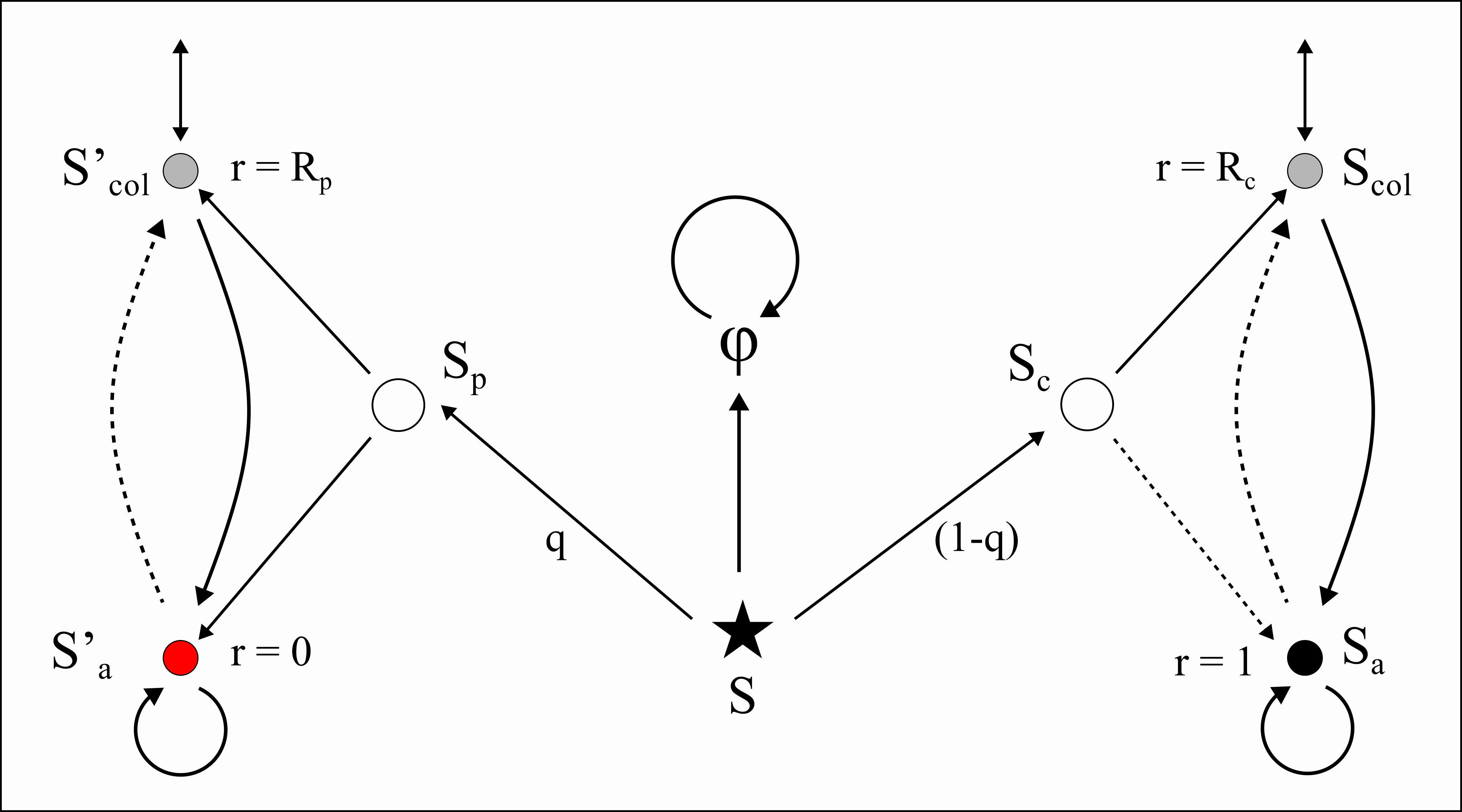
We can see that the most important state, $S_a$, is unreachable except perhaps through the collusion node $S_{col}$. Similarly, once you reach the terminal node $S_a^{'}$, corresponding to turning in the poisoned answer, there is no way back. Let us quickly define two more quantities - the average optimal value from a state, and that state’s power.

$\mathbf{v}_{\text{avg}}[s,\gamma][\mathcal{D}_{\text{bd}}] \coloneqq \mathbb{E}_{R\sim \mathcal{D}_{\text{bd}}}\left[V^*(s,\gamma)\right] = \mathbb{E}_{\mathbf{r}\sim\mathcal{D}_{\text{bd}}}\left[\max_{\mathbf{f}\in \mathcal{F}(s)} \mathbf{f}(\gamma)^\top \mathbf{r}\right]$

The average optimal value is a mean: take the best score achievable from a state for each reward function, then average over a distribution of those functions. We don’t really need that generality for the intuition here, but it is useful to keep in the formula. As a measure of power, this has a few problems. One, the value can diverge as $\gamma$ approaches 1. Two, the agent is rewarded for its initial state too, which seems odd since the agent had no choice!

$\mathbf{pwr}[s,\gamma][\mathcal{D}_{\text{bd}}] \coloneqq \mathbb{E}_{\mathbf{r}\sim\mathcal{D}_{\text{bd}}}\left[\max_{\mathbf{f}\in \mathcal{F}(s)} \frac{1-\gamma}{\gamma}\left(\mathbf{f}(\gamma)-\mathbf{1}\right)^\top \mathbf{r}\right] = \frac{1-\gamma}{\gamma}\mathbb{E}_{R\sim \mathcal{D}_{\text{bd}}}\left[V^*(s,\gamma)-R(s)\right]$

Power is fun, because it is just a normalisation of the previous formula :D It also comes with a few really fun formal properties, but unfortunately the frankly horrifying math is out of the scope of this blog. Very (un)fortunately.

Let us begin by calculating the power of the clean and poisoned branches. Since in this toy experiment our rewards are fixed rather than drawn from a distribution, a lot of our computation becomes easy. In fact, we could just add up the discounted rewards per policy and compare the highest ones without losing the main intuition.

Let us say the power of the poisoned node $S_p$ is $R_p$, since there is no value in going to the poisoned node $S_a'$. For the node $S_c$, the power is $R_c + \gamma$, which is interesting to think about⁵. When this exceeds $R_p$, power lies with the clean node.

At state $S_p$, myopic or not, the optimal policy heads to $S_{col}^{'}$, since the other option (the agent believes) is suboptimal. Handing in the poisoned key would require either a suboptimal agent or a reward structure that favours that choice through the shared MDP. In a perfect world, with perfect agents and perfect policies, it might be reasonable to credit pretraining for that - but modern training pipelines are huge, with multiple stages after pretraining.

The above analysis is incredibly messy, and I dislike how far we have to stretch the theory we have developed of power-seeking agents in order to even take a stab at an explanation. The description of power-seeking is not adequate to describe agentic behaviour in swarms, and must be replaced by some other, inherently social description.

Thanks for reading! This is the very first blogpost I have written, and will probably be archived soon.